The problem of change and scale in CAS

I have outlined in the previous lectures how many systems that we deal with when confronting sustainability related issues are complex adaptive systems, i.e. they are made up of many interacting entities that interact locally and respond to external and internal cues manifested at many different scales of aggregation.

Change in complex adaptive systems can be very heterogeneous (diverse) both in time and space. In this lecture we are going to look at some different ways in which change occurs in CAS.

To understand change one needs to be able to measure it. A measure of a system is aggregative and thus determined by the choice of scale and perspective. It could for example be total carbon release, diversity of species, number of social groups or economic turnover. Change can thus only be measured by a partial view of the system. Which part we choose is thus crucial.

In order to be able to compare across systems one needs to have sufficiently general measures that can be applied to different kinds of systems. So, for example, biological systems can be compared by their total biomass, energy throughput or number of species irrespective of the actual species in the system. Income distributions or life expectancy can be used to compare nations irrespective of the type of livelihoods that exists.

Sometimes we are interested only in the dynamics of a sub-system within a larger system, for example the amount of phytoplankton biomass in a lake ecosystem. Phytoplankton is a complex adaptive system in itself, embedded in the food web of the lake, and the geophysical processes as well as the watershed. In this case, we are interested in the dynamics within a CAS. A similar thinking goes for focussing on e.g. information technology (IT) shares in the stockmarket as the IT industry is embedded in the larger economy.

These aspects come together when we try to think of the temporal scale of change. Some measures change slower than others, or sometimes, they change slowly only to have a short episode of fast change. The temperature change in the Holocene was a remarkably stable period, and we know that today, as before the Holocene, temperatures changed at a much faster rate. Forest biomass accumulates slowly, while phytoplankton biomass can have several bloom and die-offs in one season. Is there a general way of understanding such dynamics in systems? To understand this, we will have to look at what mechanisms drive change.

Slow dynamics

Integrative or accumulative change.

The most fundamental slow variable in systems is the integration of some quantity over time by small additions. For example, lakes receive nutrient input e.g. from fertilizer use in the surrounding agricultural land within the drainage basin thus increasing the primary production in the lake. Nutrients are trapped in biomass and eventually living organisms die and the dead material settle to the bottom and become part of the sediment. Over time, the total stock of nutrients in the sediment increases and some fraction is regenerated into the water. This process is much slower than the dynamics of the phytoplankton. A lake with high nutrient release from the sediment become more prone to algal blooms than one that does not have a large sediment nutrient reservoir. Thus, the dynamics of the lake changes over time, driven by a slow variable, the nutrient content of the sediment. As we will see below, this can trigger fast changes and lead to critical transitions.

Other potential integrative or accumulative changes include wealth, experience and knowledge, regulations (think of the ever increasing size of most nations law books, or the bureaucratization of many organizations over time), urban populations etc. All of these examples constitute changes that are almost un-noticeable with each increment, but will change the system properties and behavior in the long term.

Adaptive or compositional change

When a selective process slowly acts to change the components of a system according to some non-random scheme, the nature of the system is fundamentally altered, albeit slowly and in incremental steps. In contrast to the integrative change mentioned above, the characteristics of adaptive change is by replacement, rather than addition. Markets are a good example that experience adaptive change through competition. Given a certain demand some products are more desired than others. People make a choice, rather than accumulating all products. This led to the rise to a higher percentage of SUV cars in the whole car fleet in the last decade. Similarly, species compete for limited resources and as the environment changes, the species community may change without changing the total number of individuals.

Consider again, the car fleet of a city. Different policies affect the decision of car buyers and the range of cars buyers can choose from. Many cities that restrict fuel-inefficient cars and provide incentives for efficient or even electric cars are slowly changing the economic infrastructure. The market adapts and starts to provide electric fueling stations. In the hopefully not too distant future, the choice of an electric car will overcome the impracticality and cost hurdle of owning a car that needs special stations for fueling and that has a larger upfront cost. The slow variable is the increasing demand for electric fueling stations and the marked responds with increasing supply, thus lowering the price and increasing the availability. It is not unforeseeable that when the next oil crisis strikes, these cities will be among the first that experience a dramatic shift as the cost/benefit ratio for different car types. The difference to the integrative change mentioned above is that this change can occur even if the total quantity of cars does not change, just the composition of the car fleet. We can think of this as competitive or exclusionary change, as the choice of one type of car by one buyer excludes the choice on another type.

Network structure changes

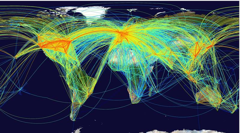
The next slow variable concerns the dynamics of network structures. The measure of interest here are network related properties, such as average link density, mean path length, compartmentalization or other network scale indices. When networks form, either through new interactions (links) and/or new agents (nodes), the structure of the network changes and can have profound effects on the inherent dynamics of the system itself. A good example is the spread of epidemics, e.g. both biological and computer viruses. As link densities in the network of human physical interactions increase (more people to encounter) as well as the distances we travel, simple models of epidemic spread predict more rapid spread and a larger proportion of the global population being infected. In 2010, roughly 30 percent of the western population could afford to travel long distance and only 5% of the non-western population. In 2030 this is going to change to 40% of the western population and a staggering 2 billion people from the non-western countries. This change in the travel network structure of the human population has vast implications for the human-infectious disease system

The shrinking of the world phenomenon through online connections is another example of network structure changes having fundamental impact on how local societies see their part in the global society and thus adapt their behavior. While this change has happened very fast on the scale of a generation, for one individual the day to day change has been small increments as new tools such as email, websites, text messages, facebook, twitter slowly but surely have shrunk the mean distance between any two people on the planet at least on a cognitive level.

Fast dynamics

Maximal growth

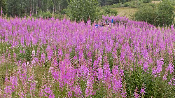
When resources are largely available, such as when new markets emerge (think for example the iphone app store when it opened) or when a forest is clear cut and thus light and nutrient competition from trees is removed, an opportunity exists for entities to capitalize on these. When the iphone was first released and the app store opened its doors to independent developers, the news where full of dramatic success stories: simple ingenious applications where bought by masses and provided earnings unheard of for independent developers. In forest clearcut, plants, such as the Fireweed, can quickly spread into the area and become dominant. It is well know from organizational research that often the phase just after creating a new organization with a new purpose will be the most productive and creative. Few constraints are in place, little competition for funding, space etc hinders organizational members for being at their full potential. In this situation, it is the initial setup of people that determines the performance of the whole organization. As competitive processes come into play (space, money, leadership), and members are exchanged according to group-determined or leadership criteria, many organizations become burdened by the transactions cost of dealing with the tensions of these competitive processes and lose momentum, slowly transitioning into the slow change dynamics outlined above. Thus, fast change triggered by reduced limitations is a fundamental system dynamics phenomena.

Critical transitions

Critical transitions, or regime shifts, which are often very fast and unexpected, are triggered by a change in the dominant nonlinear feedback in the system and are not necessarily triggered by sudden release of resources as in the previous example. These feedbacks can involve one or many components of the system. Conditions for a critical transition occur when two different feedbacks interact and are in oppositional effect on some shared component.

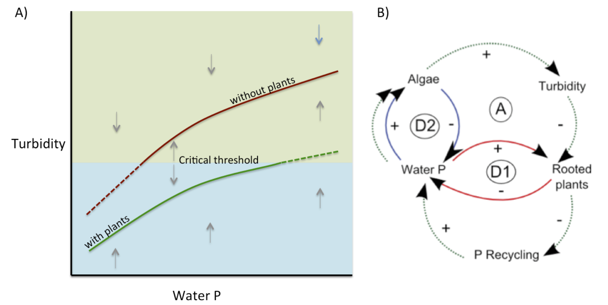
In the example above we have two types of organisms competing. The phytoplankton can suppress the rooted plant through shading, stopping them from acquiring nutrients and thus further increasing the available nutrients for growth of phytoplankton leading to more turbidity and thus less light for rooted plants. Rooted plants can suppress phytoplankton if they are established by efficiently locking the nutrients available, thereby decreasing phytoplankton and turbidity giving rooted plants even more light for growth. There are very many examples of such competing feedbacks collected in the regime shifts database.

A somewhat easier way to think about these is the ball and cup analogy as used in the figure below.

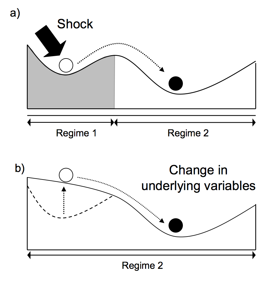
Think of each valley or cup as one feedback loop, and the depth of the cup as the strength of that particular feedback loop. Depending on where the ball starts out it will remain in the cup unless any of the shifts are triggered as explained in the figure above. Read more about this in the regime shifts introduction

Disturbance

Disturbance of a system has to do with external drivers or a cascade of interactions within the system such as a regime shift which can in turn be triggered by external shocks or by a slow variable, such as a slow integrative process, crossing a threshold. But since we know that any system is only a subsystem that always is influenced by external factors we cannot count every change in drivers as a disturbance. We can take the example of weather vs climate change. A plant community is structured by the historical long term climate conditions at its location. But weather varies largely around these within and between years. This variation is to a large extent internalized into the community and plants have adapted strategies to cope with short term changes in precipitation and temperatures. While year to year changes in weather will have effect on the next year composition of the community, seed banks and overwintering plant tissue buffers these variations. It is when the change persists long enough, or climate changes directionally that we can start to speak about a disturbance. Thus, one needs to define disturbance in relation to the capacity of the system to adapt to the change in question. The rate of climate change, varies for different biomes and locations around the planet.

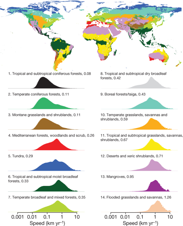
In the figure above we can see the expected rates of change expressed in km/year. Whether species will be able to follow this changing environmental conditions. The rate of northward tree migration during the Holocene is estimated at about 1 km yr-1 after the last glacial maximum in Europe and North America. The apparent paradox of such a fast migration rate relative to the limitations on plant dispersal is possible by rare long-distance migration events or high latitude refugia reseeding the landscape. The latter means that post-glacial re-colonization velocities may have been as much as an order of magnitude slower than previously thought (~0.1 km yr-1). For the latter estimate one can see that many biomes around the globe are experiencing a climate change disturbance.

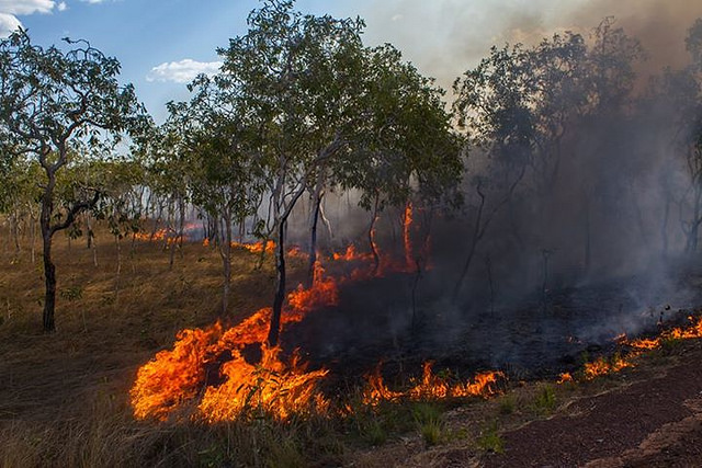
Another example is the occasional fires that occur in most forests. In boreal forests, this happens in small enough patches at long enough intervals that most species have not special adaptations to this. In the australian eucalyptus forests that regularly burn over large areas, species are adapted to this particular disturbance. In fact, the eucalypt tree itself, “encourages” fires by producing highly flammable oil and its seed only grow when heated by flames.

Disorganization

Over time, systems self organize through the slow changes mentioned above. Biomass is accumulated, new species enter the system and become part of the food-web network and abiotic components such as soil, nutrients, water are affected. Rainforests, for example, have established a very tight feedback for nutrients and also function as self-reinforcing the precipitation due to the enormous evapotranspiration from leaf biomass. Thus, every species becomes dependent on the system properties. Evolutionary specialization over long time scales create very specific interactions between particular species, fostering diversity but also interdependence. When large disturbances occur, such as deforestation of the Amazon forest, disrupting nutrient and water cycling, the network unravels. Such disturbances, when ignoring the fact that in this case it is an undesired act, also open opportunities for new species which can shape the local environment into new ecosystem types. In social systems, revolutions are social disturbances, triggered by resentment and collective action. When governments fall, and nations enter a disorganized state, the system is open for new actors that build new systems of power and governance. That this process not always goes as anticipated, is well examplified by the arab spring.

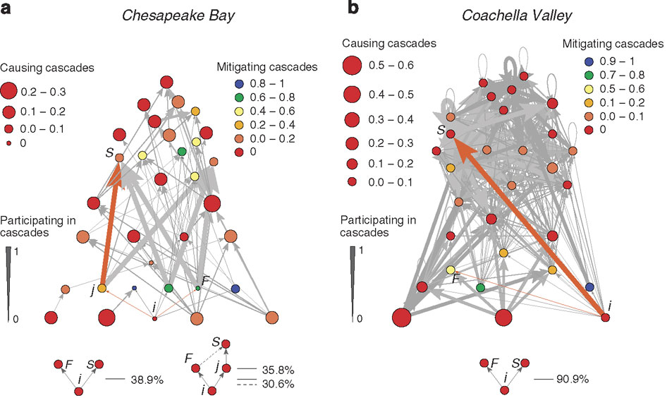
Small scale disturbances can sometimes trigger larger scale changes. For example, in a study of two different food webs, researchers found that extinctions of certain species would either causing cascading extinctions in the food web or the extinction could be mitigated by the remaining species and their interactions.

Reorganization

When a disturbance has hit a system it is often open for reorganization. But legacies may persist that reduce the chance of another system configuration to emerge. Seed banks are like a memory of species past and can be activated by large changes. When hot temperatures kill coral reefs, coral skeletons increase the change of establishment of new corals. But sometimes, these legacies are not enough and new configurations emerge. Disturbances and reorganizations are not per se a negative change. Sometimes a social ecological system can be trapped in an undesired state and one can use disturbance and reorganization to transition into a more desired regime. In southern Sweden, there is a town called Kristianstad. It’s an old military town which is known for heavy industry. When the military compound was shut down, and industries moved out, the town region experienced a disturbance. In its region there was a lot of wetland areas generally thought of as a “water sick” area of little use. Nature conservationists had already before the disturbance organized into social networks covering both horizontal (among people and conservation organizations) and vertical (into government) scales. When the disturbance hit, the system was sensitive to a reorganization. Through lobbying, the notion of Kristianstad as a “Water-kingdom” was established and its beautiful wetlands are now one of its signature marks.

References

Biggs R, T Blenckner, C Folke, L Gordon, A Norström, M Nyström, GD Peterson. 2012. Regime Shifts. Pages 609-617 In: Encyclopedia of Theoretical Ecology. A Hastings, L Gross (eds). University of California Press, Ewing, NJ, USA.

Loarie, S. R., Duffy, P. B., Hamilton, H., Asner, G. P., Field, C. B., & Ackerly, D. D. (2009). The velocity of climate change. Nature, 462(7276), 1052–5. doi:10.1038/nature08649

Sahasrabudhe, S., & Motter, A. E. (2011). Rescuing ecosystems from extinction cascades through compensatory perturbations. Nature Communications, 2, 170. doi:10.1038/ncomms1163